
티스토리 뷰
인공지능을 위한 선형대수 - CHAPTER 3.2 Least Squares와 그 기하학적 의미
developer0hye 2020. 11. 5. 19:24https://www.boostcourse.org/ai251/lecture/540328?isDesc=false
인공지능을 위한 선형대수
부스트코스 무료 강의
www.boostcourse.org
Geometric Interpretation of Least Squares
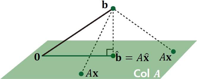
Least Squares는 \(||\mathbf{b} - \hat{\mathbf{b}}||\)를 최소화 할 수 있는 \(\hat{x}\)을 구하는 방법입니다. 여기서, \(\mathbf{b}\)는 우리가 피팅하고자 하는 Ground Truth 벡터이고 \(\hat{\mathbf{b}}\)는 우리의 모델 \(A\hat{x}\)로부터 예측되는 벡터입니다. \(\hat{\mathbf{b}}\)는 죽었다 깨어나도 Col(A) 를 벗어날 수 없습니다. 위 그림을 바탕으로 \(\hat{\mathbf{b}}\) 를 Col A 상에서 요리 조리 움직여 봤을때, \(||\mathbf{b} - \hat{\mathbf{b}}||\)는 \(\mathbf{b} - \hat{\mathbf{b}}\)가 Col(A)에 수직할때 최솟값을 가진다는 것을 파악할 수 있습니다.
\(\mathbf{b} - \hat{\mathbf{b}}\)가 Col(A)에 수직하면, \(\mathbf{b} - \hat{\mathbf{b}}\) 와 Col(A) 의 모든 벡터의 내적은 그 값이 0이 나와야 합니다. \(A\mathbf{x}\) 에서 어떤 \(\mathbf{x}\) 가 오든지간에 \(A\mathbf{x}\) 와 \(||\mathbf{b} - \hat{\mathbf{b}}||\) 의 내적이 0 이라는 의미입니다.
Column의 사이즈가 n 인 행렬 \(A\) 의 Column vectors 를 \(\mathbf{a}_{1}\), \(\mathbf{a}_{2}\), ... , \(\mathbf{a}_{n}\) 라고 하고, Column Vector \(\mathbf{x}\) 의 원소를 \({x}_{1}\), \({x}_{2}\), ... , \({x}_{n}\) 라고 정의하겠습니다.
그러면, \(\mathbf{b} - \hat{\mathbf{b}}\)와 Col(A)이 수직할때의 내적 값을 아래와 같이 표현할 수 있습니다.
\( (\mathbf{b} - \hat{\mathbf{b}}) \ \bot \ A\mathbf{x} \Rightarrow (\mathbf{b} - \hat{\mathbf{b}}) \ \cdot \ A\mathbf{x} = 0 \)
여기서 \(A\mathbf{x}\) 를 \(\mathbf{a}_{1}{x}_{1} + \mathbf{a}_{2}{x}_{2} + \dots + \mathbf{a}_{n}{x}_{n} \) 으로 전개할 수 있습니다.
\((\mathbf{b} - \hat{\mathbf{b}}) \ \cdot \ (\mathbf{a}_{1}{x}_{1} + \mathbf{a}_{2}{x}_{2} + \dots + \mathbf{a}_{n}{x}_{n}) = 0 \)
\((\mathbf{b} - \hat{\mathbf{b}}) \ \cdot \ \mathbf{a}_{1}{x}_{1} = 0 \)
\((\mathbf{b} - \hat{\mathbf{b}}) \ \cdot \ \mathbf{a}_{2}{x}_{2} = 0 \)
...
\((\mathbf{b} - \hat{\mathbf{b}}) \ \cdot \ \mathbf{a}_{n}{x}_{n} = 0 \)
위식에서 \({x}_{1}\), \({x}_{2}\), ... , \({x}_{n}\) 가 어떤 값이든 \((\mathbf{b} - \hat{\mathbf{b}}) \ \cdot \ \mathbf{a}_{k}{x}_{k} = 0 \) 가 0이 돼야하므로 \({x}_{1}\), \({x}_{2}\), ... , \({x}_{n}\) 들은 식에서 소거해줍시다.
\((\mathbf{b} - \hat{\mathbf{b}}) \ \cdot \ \mathbf{a}_{1} = 0 \)
\((\mathbf{b} - \hat{\mathbf{b}}) \ \cdot \ \mathbf{a}_{2} = 0 \)
...
\((\mathbf{b} - \hat{\mathbf{b}}) \ \cdot \ \mathbf{a}_{n} = 0 \)
여기서, 내적 연산(inner product 혹은 dot product)을 풀어쓰면
\( \mathbf{a}_{1}^{T} (\mathbf{b} - \hat{\mathbf{b}}) = 0 \)
\( \mathbf{a}_{2}^{T} (\mathbf{b} - \hat{\mathbf{b}}) = 0 \)
...
\( \mathbf{a}_{n}^{T} (\mathbf{b} - \hat{\mathbf{b}}) = 0 \)
가 됩니다. 그리고! \(\hat{\mathbf{b}}\) 을 \(A\hat{\mathbf{x}}\) 로 풀어쓰면~
\( \mathbf{a}_{1}^{T}(\mathbf{b} - A\hat{\mathbf{x}}) = 0 \)
\( \mathbf{a}_{2}^{T}(\mathbf{b} - A\hat{\mathbf{x}}) = 0 \)
\( \vdots \)
\( \mathbf{a}_{n}^{T}(\mathbf{b} - A\hat{\mathbf{x}}) = 0 \)
라는 식들을 구해낼 수 있습니다.
그리고 위식은 아래와 같이 행렬과 벡터간의 곱으로 나타낼 수 있습니다.
\( A^{T}(\mathbf{b}-A\hat{\mathbf{x}}) = 0 \)
여기서 0은 스칼라 0이 아닌 벡터입니다!
Normal Equation
\( A^{T}(\mathbf{b}-A\hat{\mathbf{x}}) = 0 \)를 전개하면 다음의 수식이 성립합니다.
$$ A^{T}A\hat{\mathbf{x}} = A^{T}\mathbf{b} $$
위 수식은 Normal Equation이라고 불립니다.
그리고, 위 수식은 새로운 Linear System으로 해석가능합니다. \(C\mathbf{x} = \mathbf{d} \), 여기서 \(C\)는 \(A^{T}A\) 이고 \(\mathbf{d}\)는 \(A^{T}\mathbf{b}\)입니다.
만약 \(C = A^{T}A\)가 Invertible 하다면, Solution은 다음과 같이 계산될 수 있습니다.
$$ \hat{\mathbf{x}} = (A^{T}A)^{-1}A^{T}\mathbf{b} $$
\(\hat{\mathbf{x}}\)이 Least Squares를 통해 구해지는 Solution입니다.
정리하면 Least Squares 방법은 \(A\mathbf{x} \simeq \mathbf{b}\)인 Linear System에 대하여 Solution \(\hat{\mathbf{x}}\)를 구함에 있어, \(\mathbf{b}-A\hat{\mathbf{x}}\)가 Col(\(A\))에 수직이되는 Solution을 찾는 방법입니다.
'Math > Linear Algebra' 카테고리의 다른 글
| 인공지능을 위한 선형대수 - CHAPTER 3.4 Orthogonal Projection 1 (0) | 2020.12.08 |
|---|---|
| 인공지능을 위한 선형대수 - CHAPTER 3.3 정규방정식 (0) | 2020.11.14 |
| 인공지능을 위한 선형대수 - CHAPTER 3.1 Least Squares Problem 소개 (0) | 2020.10.24 |
| 인공지능을 위한 선형대수 - CHAPTER 2.7 전사함수와 일대일 함수 (0) | 2020.10.24 |
| 인공지능을 위한 선형대수 - CHAPTER 2.6 선형변환 with Neural Networks (0) | 2020.10.22 |
- Total
- Today
- Yesterday
- 인공지능을 위한 선형대수
- 위상 정렬 알고리즘
- PyCharm
- 백준 1766
- C++ Deploy
- 이분탐색
- 가장 긴 증가하는 부분 수열
- 백준 11437
- 백준
- cosine
- MOT
- LCA
- 문제집
- 파이참
- 조합
- 백준 11053
- FairMOT
- 순열
- Lowest Common Ancestor
- ㅂ
- 단축키
- 백트래킹
- 자료구조
| 일 | 월 | 화 | 수 | 목 | 금 | 토 |
|---|---|---|---|---|---|---|
| 1 | 2 | 3 | 4 | |||
| 5 | 6 | 7 | 8 | 9 | 10 | 11 |
| 12 | 13 | 14 | 15 | 16 | 17 | 18 |
| 19 | 20 | 21 | 22 | 23 | 24 | 25 |
| 26 | 27 | 28 | 29 | 30 | 31 |